
The development of an economically efficient drilling program in shale-gas plays is a challenging task, requiring a large number of wells; even with many wells, the average well production and the variation of well performance (economics) remain highly uncertain. The ability to delineate a shale play with the fewest number of wells and to focus drilling in the most productive areas is an important driver of commercial success. Here, we present a new methodology for improving the economic returns of shale-gas plays.
Introduction
The methodology proposed in this study informs the development of drilling policies for shale-gas opportunities by use of a probabilistic model that accounts for the uncertainty in the chance of success (COS) and its spatial dependency. The model developed in this study shows how a prior view of the COS across a shale-gas play is updated as more wells are drilled. Inferred chances of success of undrilled well locations allow decision makers to react to newly arriving well data and optimize the development of a shale-gas resource.
The main contributions of this paper are (1) to establish and quantify any spatial dependencies between the performances of shale-gas wells, an assessment based upon data from the Barnett shale; (2) present a comprehensive method for updating COS probabilities consistently with the arrival of new information in a play with spatial dependencies; and (3) demonstrate the approach through an analysis of data from the Barnett shale.
For a discussion of previous work performed in uncertainty resolution in inconventional gas plays, including the role played by spatial dependency, please see the complete paper.
Shale-Gas Economics in the Study Area
Well Data. The investigated area is located in the eastern part of the Mississippian Barnett shale in the Fort Worth basin in Texas (Fig. 1 above). The study area covers 2100 km2 and straddles Johnson, Tarrant, and Ellis Counties. A set of 2,901 horizontal wells has been analyzed; 2,064 of these are located in the “Training” area (see later reference in this subsection). Well data include well location; date of completion; first 6-, 12-, or 24-month cumulative gas production; and the length of the well. The data originate from the US Energy Information Administation (www.eia.gov).
The first horizontal wells in the investigated area were drilled in 2003. After a slow uptake in 2003 and 2004, the number of wells drilled per year strongly increased until 731 wells were drilled in 2008. Over the following 2 years, the number of wells drilled per year dropped to less than 650 wells.
This area has been divided into northern and southern halves. The southern area is referred to as the Training area, and the northern area is referred to as the Test area. Data from the Training area will be used to define geostatistical parameters that will be applied subsequently to data from the Test area.
For a detailed discussion of type-curve modeling and cash-flow analysis for the analyzed wells, please see the complete paper. The complete paper also discusses the determination, by use of geostatistical analysis, of spatial dependencies in the Barnett shale.
Method for Updating COS As New Wells Are Drilled
The method developed in this study aims to provide insight into the geographical variation of the COS and into how the view of COS evolves as more well data become available over time. The maximum entropy principle is used to develop an initial view of the COS of a cell, then to perform a Bayesian update (BU) when the results of new drilling within it become available; finally, the impact of that new information is propagated to nearby cells by use of geostatistics [in this case, indicator kriging (IK)]. This will be referred to as the BU-IK method. The overall process consists of three steps.
Step 1. Before any well data are available in the play, a probability-density function (PDF) for COS is assigned to all cells. (Strictly speaking, a discrete distribution, a probability mass function, is used for COS. However, because practitioners are more familiar with the term PDF, this term is used throughout this paper.) This is the prior distribution, which should be based on all information available up to that point. The prior knowledge typically comes from analog plays and specific information about the current play, as well as general geological and reservoir knowledge.
Step 2. At some point in time, new well information arrives in the form of well successes or failures within a cell. Bayes’ rule is then used to update the PDF in the cells where wells have been drilled. This results in new PDFs (posteriors) in all cells with new well information. These posteriors are based on the combination of the prior uncertainty and the new information. In the cells for which there are no new wells, there is no change to the PDFs. These cells will be updated in Step 3.
Step 3. Given the spatial dependencies in the play, one would expect cells that were not updated in Step 2 and that are adjacent to cells for which there were significant changes to the PDF to be affected by these changes. In this step, this spatial dependency is taken into account and IK is used to update the cells that were not updated in Step 2.
Upon completion of Steps 2 and 3, all cells in the play have been updated and the posterior distributions in the cell account for all available information. If new well information arrives subsequently, this posterior will be used as the new prior, and Steps 2 and 3 will be repeated.
For a detailed discussion of this process, as well as the details of each step in the calculation procedure, please see the complete paper.
Illustrative Application to the Barnett Shale
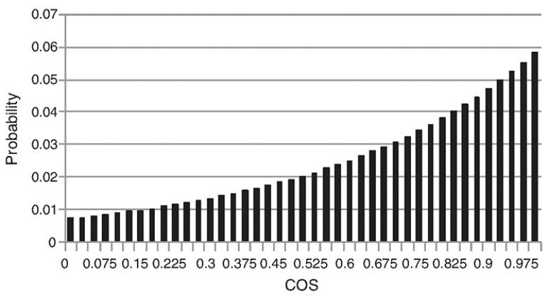
Predrilling Information. The COS determined on the basis of all wells in the Training area is assumed to be the prior COS of the Test area. The percentage of wells that had been drilled in 2011 that yield a positive net present value assuming a gas price of USD 4/Mscf amounts to 67.2%. Hence, 0.672 is taken as the prior COS. The maximum entropy principle is used to develop a probability distribution of COS (Fig. 2). (Alternatively, one could have used the probability distribution based on the well results from the Training area.) This probability distribution has been assigned to each cell. The assumption is made that 40 wells can ultimately be drilled in each cell. This assumption implies a well spacing of 0.16 km2 per well (or 40 acre/well).
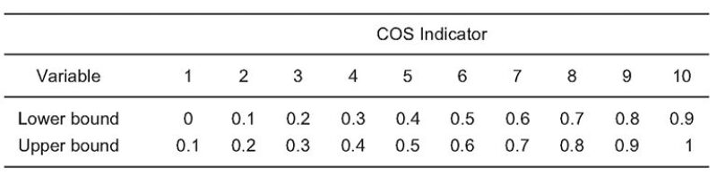
Variogram for Ordinary IK. Ten COS indicators have been defined. The lower and upper bounds for the indicators are listed in Table 1. Data from the Training area have been used to develop experimental variograms for each indicator. In all ten of these variograms (Fig. 16 of the complete paper), a nugget effect can be observed, and five variograms are dominated by the nugget effect.
COS Based on Realized Well Data
The map shown in Fig. 3 presents the observed COS values in the Test area based on data from the 837 wells that were drilled before Q2 2011. The region with the highest COS is located in the southern-central part of the study area. The authors use the map in Fig. 3 to represent the “true” distribution of COS in order to test the predictions generated by the Bayesian-kriging method that are based on (significantly) fewer well data.
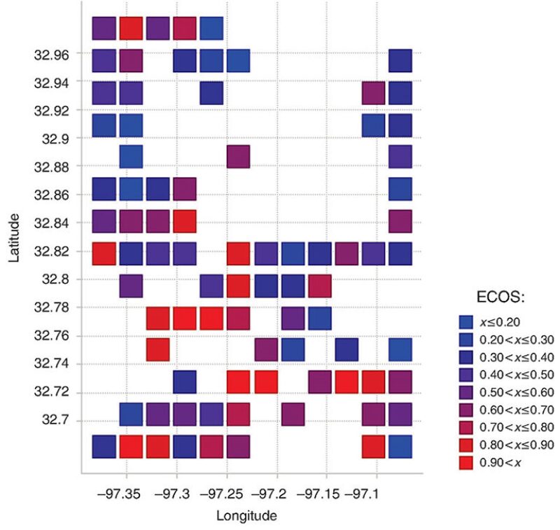
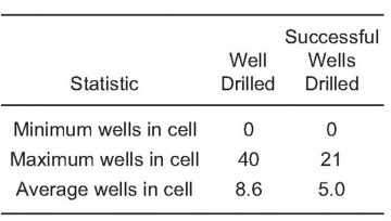
By Q2 2011, 92 out of a total of 168 cells had been drilled. The statistics on the number of wells in the cells are summarized in Table 2.
Results
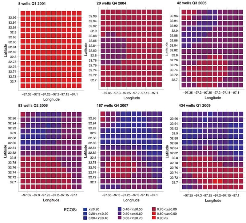
The authors show how the view of the play changes as progressively more well data become available over time. For simplicity, rather than try to show the full COS PDF for each cell, the authors will use the expected COS (ECOS) derived from the COS PDF. The panels in Fig. 4 track the development of the view on the spatial distribution of ECOS. A comparison of the regional variation of observed COS on the basis of all available well data from the Test area (Fig. 3) and the inferred regional variation of ECOS shown in the panels of Fig. 4 shows that much of the general outline of the variation of COS was defined after the first 187 wells were drilled. The southeast/northwest-trending anomaly of high COS values in the southern part of the Test area (Fig. 3) can be inferred from the first 187 wells (Fig. 4). The addition of more than 1,200 wells, to a total of 1,489 wells, does not change the geographical variation of COS significantly.
Discussion
Spatial Dependencies and Nugget Effect. Variograms from the eastern part of the Barnett shale suggest that significant spatial dependencies between shale-gas wells do exist. In most of the calculated variograms, sills can be defined at a lag of 15–20 km. This suggests that spatial dependency exists between wells that are spaced 15–20 km apart.
A relatively large nugget effect suggests the presence of a large localized variation. This local variation is probably a combined effect of small-scale geological features and uncontrolled variations in well completions and operations.
It has been suggested that well performance in the Barnett shale changes significantly with depth and formation thickness. The nugget effect present in the variograms presented in this study could potentially be reduced by accounting for these and possibly other factors that affect the variability of well performance.
Reacting to New Information. Continuously updated understanding of key uncertainties could affect the strategic decision making during the development of a play. Drilling programs in areas that outperform a prior expectation might be accelerated, while drilling in areas with disappointing results might be abandoned. Although one might expect that drilling over time would be concentrated in the high-COS areas, there appears to be little evidence for such a trend in the analyzed data from the Barnett shale. It is possible that contractual obligations have prevented such economic optimization. For example, in the Haynesville shale, high drilling activities persisted in 2010 and 2011 despite low gas prices. Some authors have anticipated that, once these drilling obligations have been fulfilled, economic considerations will define future drilling activity. Historically higher gas prices might also provide an explanation. Areas that are not economical at USD 4/Mscf might have been economical when they were initially developed, when gas prices were significantly higher. The currently perceived need to optimize what areas to develop might not have been as great if all considered well locations were yielding positive economic returns.
Conclusions
Well-to-well correlation is an important aspect of the valuation of unconventional gas plays. The analysis of Barnett shale data suggests that despite local variations in well performance, significant dependencies between proximate cell locations do exist. Furthermore, these dependencies can be exploited by standard geostatistical techniques to predict well performance at undrilled locations. The proposed approach propagates the updates to nearby cells, allowing decision makers to update their prior view on expected well performance at undrilled locations when additional well data become available.
Through the application of the BU-IK approach, cell-to-cell COS dependencies can be expressed as a function of spatial separation between two cells. This enables efficient determination of dependencies for a large number of drilled wells and possible well locations.
This article, written by JPT Technology Editor Chris Carpenter, contains highlights of paper SPE 164816, “Combining Geostatistics With Bayesian Updating To Continually Optimize Drilling Strategy in Shale-Gas Plays,” by B.J.A. Willigers, BG Group; S. Begg, University of Adelaide; and R.B. Bratvold, University of Stavanger, prepared for the 2013 EAGE Annual Conference and Exhibition incorporating SPE Europec, London, 10–13 June. The paper has not been peer reviewed.