
During hydraulic fracturing, pumping data is recorded and mapped in the field at one-second intervals and saved in comma-separated files (.CSV). The raw pumping data includes multiple data channels, including treating pressure, slurry rate, clean volume, and proppant concentration. Once the data is gathered, a field engineer manually picks events such as start and end times, breakdown pressure, instantaneous shut-in pressure (ISIP), and diverter drop from the treatment plots (Fig. 1). This manual process is time consuming, prone to error, and less reliable because of differing interpretation methods across the industry. To address this challenge, a Denver-based oilfield technology company is using machine learning to identify flags in high-frequency treating plots more accurately and consistently.
Click here to watch a presentation of Events Recognition on Time-Series Data by Well Data Labs.

data channels recorded at one-second intervals during
pumping and several event flags.
Methodology
The goal is to automate the event-picking process by training an algorithm against a large and diverse data set that has been labeled with the most common interpretations without explicitly programming it. For this, the raw data (.CSV files) are collected through cloud-based software that standardizes naming conventions and units, providing a clean data set and an efficient and effective way to visualize treating plots for optimal stage selection.
In approaching this problem, the team uses binary classification to build a model that distinguishes points, each labeled as 0 or 1. Fig. 2 shows an example of how this method is used to label the data that belongs to the stage pumping time (1s) and that which does not belong (0s). The data, which consist of features (independent variables) that are used by the model to predict the labels (dependent variable), are split into three data sets: training, validation, and test. The training algorithm builds a model that takes advantage of patterns and trends identified in the training data to classify (label) points accurately.

end time flags and the binary classification tags added
to the training data.
The validation data set, which has the same format as the training data but with fewer stages, provides an unbiased evaluation of various models constructed on the training data. The 0/1 predictions generated on the validation data set are used to build a confusion matrix and derive accuracy, precision, and recall. High accuracy, precision, and recall values are fundamental to accurate predictions. The test data set is used to evaluate the final model (and procedure) for predicting the final location of the flags. It has the same features as the training and validation set but different stages and is labeled with the correct location of the flags but not with the binary classification column. The complete work flow is shown in Fig. 3.

Start/End Flags
The designation of the stage start and end flags is critical because these boundaries govern summary calculations for that stage. The interval between the flags identifies the appropriate data to include when calculating the average and maximum pressures, rates, and concentrations, in addition to defining the cumulative volumes and pumping time, among others. For this process, the team uses treating pressure, slurry rate, and clean volume as the initial features to train a logistic regression classifier. The pumping data set consists of 179 stages, for a total of 1,530,445 rows of data per variable. Sixty-six percent of the data trains the model, 8% validates it, and the remaining 26% tests it. All three data sets include a variety of stages: some clean “textbook” stages with obvious start and end times and other “messy” stages beginning or ending with unusual behavior, which makes locating the start and end times much less clear.
Identifying the start and end times is achieved by taking the difference between consecutive rows of the predicted binary labels. Start times are identified when the difference is positive (labels switch from 0 to 1) while end times are identified when the difference is negative (labels switch from 1 to 0). This combined prediction and post-processing procedure (taking differences) generates a list of matched start and end times. Each matched pair of events is tagged with the position of the changes, the associated job time, the well name, and stage number. Then, some final filtering is applied to select the most appropriate predictions for each stage. Even though the first group of trials produced models that predict the 0/1 labels very accurately, the combined procedure generated a long list of predictions. The procedure recognized any minor change of slurry rate and pressure as a start time and assigned a corresponding end time (Fig. 4). Thus, additional features and applied techniques are added to reduce the number of false matched pairs generated.

Fig. 4—Fracture treatment plot displaying multiple
start- and end-time flag predictions.
In the second round of model training, the features are preprocessed using a simple moving average to smooth the data. The moving average transforms the time series to better highlight changes in trend by reducing minor fluctuations (noise). The team adds rates of change as additional features and applies L1-regularization to the model training. L1-regularization is often used in logistic regression to produce models that ignore less-relevant features. The resulting models tend to be more robust and easier to interpret. The final logistic regression model has a training and validation accuracy of approximately 90% while the placement of the flags on the test set are within 10 seconds of the manually selected flags on average (Fig. 5).

Fig. 5—Fracture treatment plot displaying the final
and accurate start- and end-time flag predictions.
ISIP Flags
ISIP is defined as the difference between the final injection pressure and the drop in pressure caused by friction in the wellbore and perforations or slotted liner. The ISIP flag is placed at the end of the stage pumping time, immediately after shut-in and before the pressure starts to drop. This is estimated by placing a straight line on the early pressure decline and locating the point in time where the pressure rate is zero. ISIP picks have varied in the industry as data collection becomes more and more constrained. Quite often, data collection ceases after the pumps are shut down to save operational time (and, therefore, money). Thus, only a few seconds are recorded after the rate is zero, making it very difficult to place a straight line because there is no pressure decline. For this reason, many field engineers pick ISIP at the first or second spike of the water-hammer effect observed at shut-down, making this process inconsistent.
For ISIP, 870 stages of standardized data were collected from basins all over North America through a cloud-based software application. Using a similar binary classification scheme as previously described (Fig. 6a), a neural network was trained to identify and isolate the area of the treating pressure plot needed to calculate ISIP. Points are labeled with 1s if they belong to the target area of the treating pressure plot and 0s otherwise. When the neural network identifies the target region, the time-series is further truncated by removing outliers. For this procedure, outliers are identified as points that are more than one standard deviation from the average pressure value of the isolated region. Finally, linear regression is applied to the reduced time series to predict the ISIP value when the slurry rate is zero (Fig. 6b).


Credit: Paper SPE 197093.
Fig. 6—Fracture treatment plot showing
(a) the binary classification tags added
to the training data to isolate the area
of the treating plot needed to calculate ISIP
and (b) the reduced data set
with the linear regression model to find
the specific value.
The neural network achieved a classification accuracy (on the training and validation sets) of approximately 98% when isolating the target region. The subsequent ISIP predictions from the linear regression on the test data set had an average accuracy of ±72 psi and a median accuracy of ±35 psi when compared with the manually picked values (Fig. 7).
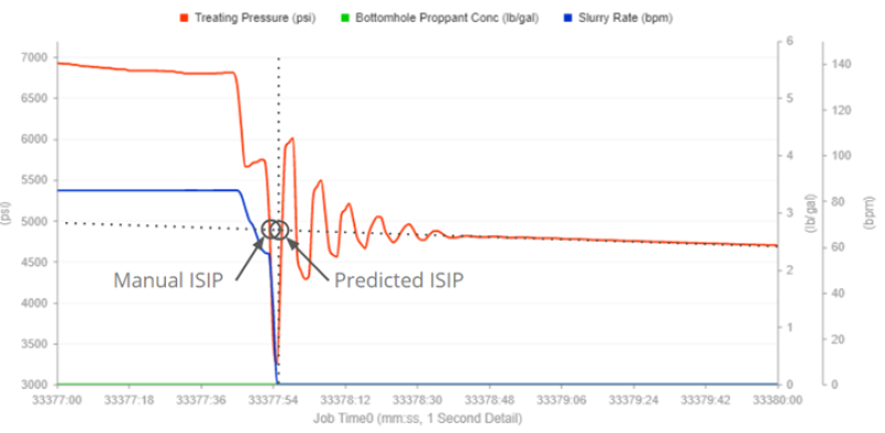
Fig. 7—Comparison between the predicted and
manually picked ISIP flags in a stage.
Takeaways
Automatically labeling relevant regions of high-frequency hydraulic fracturing treatment plots using classification techniques can lead to simple and effective procedures for identifying events of interest. Accurate flag selection makes processing large volumes of fracture treatment data viable and reduces the time spent reviewing field data for quality control. A limitation of this method is that it requires periodic retraining with new field data to maintain accuracy and improve the robustness of the prediction. The benefits of using simple (and accurate) models include ease of deployment, ease of debugging, and extremely fast prediction and retraining (updating the model).