The final act of completing a horizontal well and bringing it on line represents a special period for unconventional oil and gas producers. Typically done weeks or months after drilling and hydraulic fracturing operations, this stage—known as flowback—is akin to the moment of birth. Like a newborn baby, as each new well takes its first breath and exhales, it is customary to evaluate its health and start projecting how it will grow up.
For a shale producer, this moment weighs heavily upon its future since flowback analysis feeds into long-term recovery estimates and economic models. Flowback data are also cheap compared to many other reservoir diagnostics. The challenge lies in the fact that there is no single flowback analysis method that operators can use to land on the “right” conclusion, while locking into the wrong one can be costly.
The good news is that there are plenty of ways to narrow the band of uncertainty to paint a clearer picture of what early-time flow is really saying about how a well was completed, and what it will deliver going forward.
Several of the latest industry insights and best practices on this topic were shared last winter at a conference organized by the Calgary-based completions-focused training startup SAGA Wisdom. The firm’s first annual meeting in St. Augustine, Florida, featured a panel of reservoir engineering experts that offered candid and practical advice on how to run a flowback analysis program. The discussion reflected the shale sector’s need for data management and improved modeling methods to illuminate what really drives tight-rock production.
Components of Real-Time Flowback Analysis, With a Focus on the Full Value Chain
Improved collaboration and more integrated workflows
Pairing production analytics with fluid diagnostics (e.g., geochemistry, tracers, and RTA)
Using completion data to complement and inform interference tests
More-descriptive reservoir characterizations prior to production (e.g., on a pad-by-pad basis)
A practical and scalable toolkit
Fluid and pressure data
Building field studies and planning integrated diagnostics for the long run
Permanent downhole equipment
Increased depth of investigation
Source: James Tucker.Real-Time Flowback for Long-Term Recovery
Shale producers, service companies, and petroleum academia have delivered many flowback studies over the years. However, as far as the bottom line is concerned, flowback analysis is not merely an academic exercise. The goal for operators both large and small is to maximize rates, while minimizing the damage to the reservoir and conductive fracture networks.
James Tucker was an engineer with Devon Energy when he coauthored one of OnePetro’s most-downloaded technical papers (SPE 174831) on flowback analysis and choke management. The paper described the operator’s use of rate transient analysis (RTA) and real-time data to double 30-day initial production (IP) rates from a field in the Eagle Ford Shale in Texas.
Tucker, now a senior reservoir engineer with Austin-based Venado Oil & Gas, highlighted when the paper was written in 2014 that oil prices were significantly higher than today. That offered more leeway for engineers to test ideas with a wider margin of error than can be afforded today.
“Yes, there is value to be had by pulling the rigs forward and increasing your IP,” he said. “But as oil prices have declined, and we’ve moved to more mature plays and the second-tier areas, the range of degradation is much more sensitive.”
In other words, the sector-wide quest for high IPs has slowly given way to other metrics such as net present value and initial rate of return. Tucker illustrated this balancing act by noting that a 250 B/D increase in IP for his operating area would be “value-neutral” if that uplift resulted in an estimated ultimate recovery (EUR) degradation of just 5%. The figure puts into perspective the trade-offs between “pulling hard” on wells in their early stages vs. increasing flow over their lifetime.
Engineers at Venado are still working to describe all the driving mechanisms at play here. “We want to basically come up with a menu of options by understanding where we’re sensitive to,” Tucker said, adding that this is a work-in-progress for the majority of subsurface engineers in the shale sector which remains “fairly fragmented on what the critical considerations are.”
Some of the key areas being looked at revolve around multiphase flow, pressure-dependent permeability, and fracture conductivity. At Venado, key to deciphering how these factors play into observed reservoir responses is to watch flowback unfold in real time.
But Tucker noted that no one knows exactly what to expect during flowback. Gas-to-oil ratios might be unique, as might be water ratios. This is why strong baseline studies are required, along with quality-control practices on the data collection side.
If the data can be trusted, then the door is opened to dynamic decision making on how to flow back each well to enhance its performance. “And that allows for good collaboration,” Tucker added, noting that a firm philosophy around real-time flowback analysis narrows the debate over what to do, such as when to increase choke sizes.
The data-driven approach used at Venado also helps reduce the number of “backseat drivers” inside an organization that may otherwise influence the delicate operation. There can always be issues that hamstring a good experiment though. Flowing conditions may be great, only to outstrip takeaway capacity. Or the wells decline so fast that maintaining line pressure becomes a concern. “And that measured approach, that analysis that you did is all for naught,” said Tucker.
Tucker described the overall solution a “cyclical process where you’re constantly working with your operations group and the midstream group to get on the same page,” noting that all this begins with how the well was initially flowed back. Ideally, everything is integrated with a “practical and scalable” analytical toolkit. Looking into the future, Tucker predicted that machine learning and automation technologies will soon lead to more-efficient flowback operations.
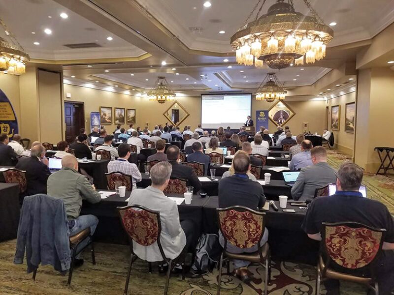
More than 70 completions experts from the US and Canada gathered in St. Augustine, Florida for a two-day conference covering some of the latest advances in unconventional completions analysis and diagnostics. Source: SAGA Wisdom.
Thinking About the “Genesis” of Data
Before diving into flowback analysis, engineers should first see the effort through the lens of data acquisition. The key ingredients include some obvious parameters: injection volumes, fluid rates, fluid properties, and pressures.
Though these are staples of the flowback data diet, for a variety of reasons, such measurements are not always reliable. If only slightly off, incorrect inputs can carry forward major impacts for those relying on correlations to estimate reservoir properties and flow behavior.
“If we’re talking RTA—if you don’t have any confidence in your rates—then don’t bother with the analysis. Just move on to more traditional things like decline curve analysis, and even then, you’re going to be struggling,” said Tyler Conner, a reservoir engineer at Oklahoma City-based Devon Energy.
One problem operators face here is that data quality issues in the field are not always obvious. But because flowback analysis is especially sensitive to bad inputs, Conner stressed that operators must “understand the genesis of your data.”
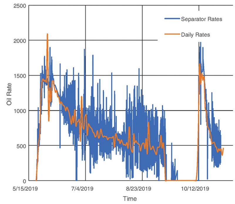
The first place to increase scrutiny is not far from the wellhead: phase separators. The upside of separators is that they usually deliver flow rate data on an hourly basis. Their drawback is that these rates can vary sharply throughout a single day, thus generating “a lot of noise” in the data, Conner said. He recommended that operators pay attention to such variability and rely on field staff to ensure that flowmeters are properly and routinely calibrated.
Aside from separators, stock tanks are also used widely across the shale sector to measure production. Unlike separators, many tank levels are reported to headquarters once a day. In addition to the lower resolution, the data collected from tanks reflects production from multiple wells on a pad. This makes allocating production figures back to a group of wells on the same pad more of an art than a science.
Conner also highlighted that the oil inside a tank is subject to significant density loss as the gas vaporizes from the emulsion, an effect known as shrinkage. This too needs to be corrected for when making flow estimates and when comparing separator rates to the daily rates taken from a tank. And once again, the advice to other operators was to communicate clearly and often with field personnel to track such changes.
“This is all stuff you need to think about before you go into any sort of analysis—you need to understand where your rate data is coming from,” said Conner.
Choosing Correlations Carefully
Beyond rates, properties of the oil, gas, and water that are collected during flowback should be analyzed properly before they are used to make predictions. Flowback analysis is so sensitive that seemingly small differences in gas and water property assumptions will yield very different bottomhole pressure estimates. Conner provided examples to make the point.
In one case, increasing the gas gravity from a default of 0.65 to 0.86 translated to an increase in bottomhole pressure of 200 psi. For produced water, upping the gravity from 1.0 to 1.1 spread the pressure estimates by 500 psi. By picking the high side in error, an operator would be at risk of overestimating a well’s long-term production.
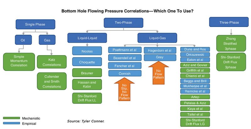
Another area for engineers to tread carefully in involves using bottomhole flowing pressure correlations to make up for a lack of downhole data. Using the same data set, and only changing the correlation for pressure drop, Conner showed how a reservoir model used to predict future reservoir drawdown over 30-years yieled two vry different estimated ultimate recovery (EUR) predictions. One was nearly double the other.
There are more than two dozen of these correlations. Some are geared toward single-phase flow, some two-phase flow, and others were designed for three-phase flow. Some account for flow patterns, but not all. “So who knows which one to use? Well, you can gather downhole gauge data to help you decide which correlation best matches your flow rates and your fluid properties,” said Conner, adding that the extra money spent will pay dividends later by preventing poor operational choices. “Be proactive about getting better data.”
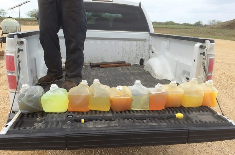
Conner also shared an image of several oil samples taken from different wells in the Eagle Ford Shale. Though each sample was taken within 5 miles of each other, the contrasting colors of each sample revealed just how different their fluid properties were.
Pressure-volume-temperature (PVT) testing would tell an operator exactly how different they are, but this is not affordable for every well. So when operators know that their crude quality comes with such variability, they are advised to be extra cautious in selecting analogues and flow correlations to model PVT properties. “You can’t take it for granted that if you have a PVT from a mile away that it is going to be anywhere near representative of a well that you’re going after now,” Conner said.
Physics-Based Flowback Analysis
A chief problem for most unconventional engineers is that to varying degrees, the initial conditions of flowback, i.e., pressure and hydrocarbon saturation near the newly created hydraulic fractures, are unknowns.
Among those tackling this problem is Chris Clarkson, a professor and Ovintiv and Shell chair in Unconventional Gas and Light Oil Research at the University of Calgary. For him, the best way to deal with this reservoir uncertainty is to use integrated modeling to simulate the hydraulic fracturing process on through flowback.
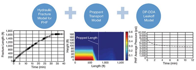
The work flow that delivers these initial conditions on flowback begins by modeling hydraulic fracture propagation and fluid leakoff during the stimulation treatment. This hydraulic fracture model also includes a proppant transport model to estimate propped fracture lengths, “and very importantly, we’re modeling the leakoff of the frac fluid during the stimulation period and the subsequent shut-in,” said Clarkson, adding that “we’re doing this somewhat rigorously” using a dual-porosity dynamic drainage area reservoir model.
From this work, Clarkson said that engineers should be able to estimate the pressures and saturations in the primary hydraulic fractures, the secondary fracture network, and the tight-rock matrix. Using an illustrative example, he showed an output of this work flow that estimated the pressures in the stimulated fractures and tight-rock matrix were more than 600 psi above the initial reservoir pressure.
“Not only are pressures elevated in this near-fracture region, but also, the fluid saturations are elevated,” he said. “We need to know this at the start of flowback, before we try to do any sort of flowback modeling. Otherwise, we could be in significant error in our analysis.”
One of the other nuances of Clarkson’s favored approach to flowback modeling involves accounting for salinity changes before and during flowback. Salinity, he said, which is modeled by coupling a salt transport model with the flowback model, provides additional model constraints that go beyond simply matching rates and pressures.
Another problem Clarkson said operators need to fully appreciate during flowback analysis is that most new horizontal wells are at some point going to communicate with neighboring offset wells. Rate transient analysis equations were developed in a conventional world, meaning they were devised as a single-well application. “However, multiwell communication is more and more prominent,” he said.
The solution that Clarkson and others have been using involves forward and inverse models—a top-down and bottom-up approach that helps build confidence in models. Key to the approach is modification of the aforementioned dynamic drainage model to account for interwell communication “that allows us to simulate flow in both the fractures and reservoir for the communicating wells,” he said. This coupling represents an emerging theme in the unconventional modeling space because it helps account for both large- and small-scale physics.
What this dynamic drainage area model allows is communication between two fractured systems from flowback to online production. Clarkson offered a use case in which the flow of six co-located wells—one upper row, one lower row—was simulated. The wells are first grouped in vertical pairings to simulate communication between them. Next, each pair then communicates with the other set of wells.
All of this is meant to drive a more realistic outcome by bringing what the sector has learned about offset wells in recent years into the modeling space. Engineers could use a model like this to extend certain RTA approaches to simulate interstage communication, which would offer an even more granular understanding of infill-well flow regimes.
Follow the Water
Robert Hawkes, a reservoir engineer and general manager of Calgary-based diagnostics firm Abra Controls, spent the early part of his career working as a reservoir engineer with pressure pumping companies BJ Services and later Trican. Looking back on his work with flowback analysis he recalled that “we always had to wrestle with why we had poor performance,” he said, adding that “the first thing we would go to would be the chemicals or a pump shutdown—and it’s easy to pick on the pumpers as we all know.”
But flowback analysis can be hamstrung in other ways. As mentioned throughout the panel, recorded pressures might not be reliable. More-accurate measurements can be acquired from downhole instruments, but again, those are cost-prohibitive for the majority of cases.
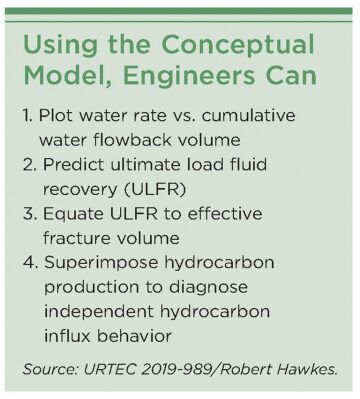
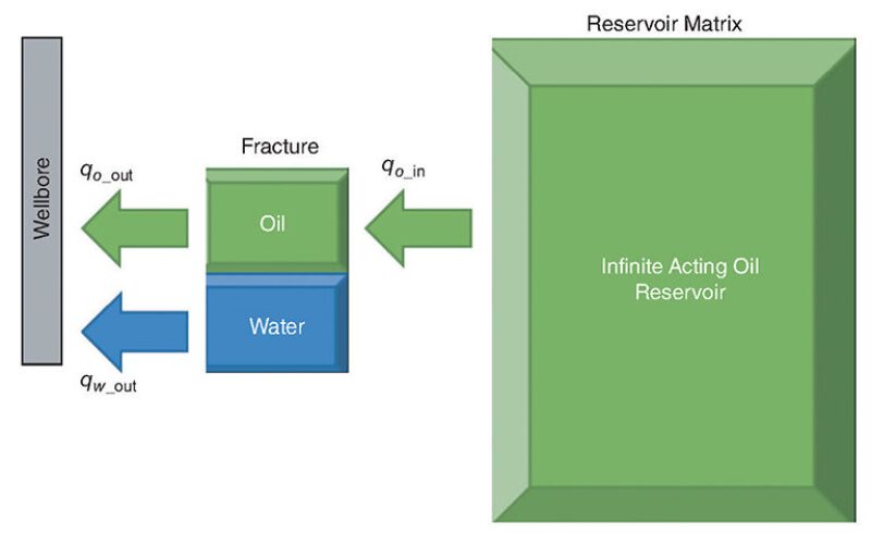
With all this uncertainty, Hawkes’ argument was to narrow the analysis. The simple approach he advocated for is the recently developed “Conceptual Flowback Model” (URTEC 2019-989) Hawkes noted that the method was developed with the help of fellow panelist Clarkson and Hassan Dehghanpour, an assistant professor of engineering at the University of Alberta.
When using the conceptual model, “I’m assuming no water production is coming from the reservoir,” during the flowback period, said Hawkes. “That’s where I start my whole interpretation process off—and that’s critical.”
This analysis holds that the fluids measured on the surface are almost entirely made of oil and gas that has flowed into the fractures after the stimulation. The gas is also independent of the water in the model. For engineers, this leaves only one key plot to follow, but it represents a “very strong signature,” Hawkes explained, adding that it helps sift through the more “noisy data” collected during flowback.
With the focus on fluid-rock interaction, the primary use case for the data becomes to estimate the effective hydraulic fracture volume. This way, wells can be compared by overlaying the analysis with longer-term hydrocarbon production.
Additionally, engineers can assess the quality of the completion, the use of surfactants, impact of choke settings, and fluid interactions within the reservoir. Hawkes also highlighted that the conceptual model reveals “dynamic changes in production” when there are workovers or significant fracture interactions between offset wells.
Underlining that operators need to apply practices tailored to their slice of reservoir rock, Hawkes said that the method has been validated using RTA and works “reasonably well” within most unconventional reservoirs.