
The low oil price era following the 2014 oil price crash created multiple concerns: an urgency to cut operating cost (OPEX), rising renewable energy competition, and growing environmental challenges. Oil and gas companies faced pressure to shift from a growth mentality to a focus on value via higher investor returns. Organic gains and free cash flows from operating assets have become more important for the short-term health of upstream oil and gas companies.
As companies have focused on giant capital investments onshore and offshore to drive growth, they have often focused less on field operations, especially OPEX. This represents an enormous opportunity to address profit squeeze by improving overall cost efficiency in oil and gas projects.
Rigorous benchmarking is a highly effective empirical tool that can shine light on overlooked opportunities and demonstrate what operating excellence looks like. Operating excellence involves balancing operating cost and safety with top-level production efficiency in a safe and sustainable manner. To achieve this goal, operators should have the right strategy for every aspect of the operations in three dimensions—cost, reliability, and health, safety, and environment (HSE). HSE performance, which is directly impacted by reliability, is not the focus of this article.
Benchmarking Is About Fair Comparison
Benchmarking has long been an effective practice to help participants find performance gaps through a series of well-defined key performance indictors (KPIs) on cost, production reliability, and HSE. Companies engage in both internal and external benchmarking exercises. The key for an effective external benchmarking is to have critical mass of peer assets for a like to like (apples to apples) comparison.
However, internal benchmarking is only marginally effective because it does not include an external view that can detect potential issues existing even in an operator’s best-performing assets. Meanwhile, direct internal comparison among different single-operator assets cannot reveal the true operating performance because there are too many independent variables. Comparing unit cost on a $/BOE basis can reveal an asset’s financial competitiveness. Since it only benchmarks cost by production and doesn’t account for asset complexity, however, it cannot measure efficiency performance.
To achieve the goal of fair comparison, the key is to address the differences among peer assets. Peer group selection and normalization are approaches used to address the “noncontrollable” operation differences among assets with the common goal—making a fair comparison on assets to reveal the operational differences in performance.
Peer group selection involves a process called common seeking, in which groups of assets with similar features are formed, such as FPSOs, fixed platforms, oil fields, gas fields, or assets in a region/basin. Meanwhile, normalization involves a process of difference identification and recognition, which addresses the feature differences among assets within a peer group. The normalization process seeks to add peers to a group by embracing feature differences, while peer group selection works to reduce peer group numbers and eliminate the feature differences. Both peer group selection and normalization are needed to successfully address the challenges in benchmarking.
How Normalization Works
For effective benchmarking, the normalization process is needed for cost, reliability, and HSE. This article will focus on two dimensions, cost and reliability.
1. Cost
Cost is a main normalization target in benchmarking. Several cost categories are generally defined in offshore operations, for example, well servicing, facility maintenance, field labor, chemicals, energy, transportation, and field general and administrative costs (G&A). Each cost category has its own cost drivers requiring separate normalization models. One KPI used to assess cost performance in a peer group is the cost efficiency index (CEI), which is the ratio of actual cost to standard cost. Standard cost is a normalized theoretical cost based on normalization and represents the average of the actual costs of assets with the same technical configuration. Generally speaking, assets with the same technical configuration share the same standard costs. Therefore, an asset with a more-complex technical configuration is given more standard cost to compensate for the higher complexity.
The concept of standard cost is the basis for valid cost-efficiency performance benchmarking. The following is a brief description of how standard cost is derived through normalization and how it is used to benchmark cost performances.
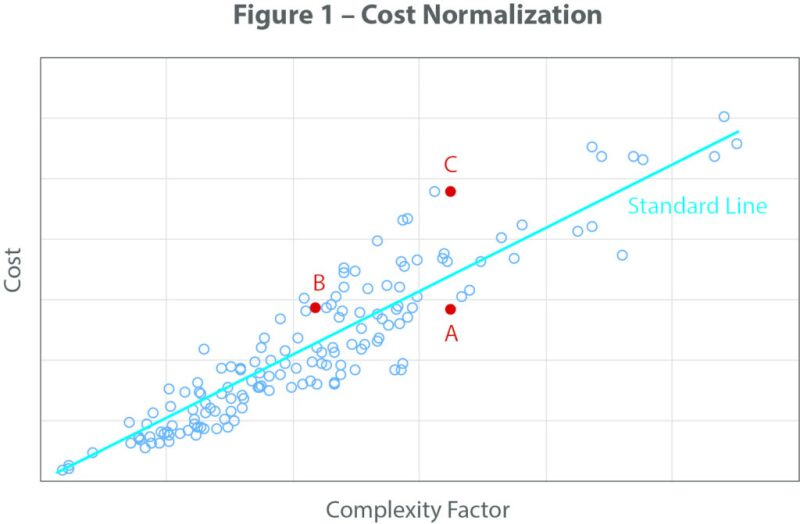
Fig. 1 demonstrates the cost- and complexity-factor relationship in a scatter chart of peer assets. The complexity factor (x-axis), which represents the operational complexity of the asset, is an aggregated value of technical configurations of the asset. The standard line, formed on the regression of actual cost (y-axis) and complexity factor, is used to derive the standard costs for assets with different complexity factors.
For example, Asset A has an actual cost of ACa = 140, and a complexity factor of CFa = 16, which relates to a standard cost of SCa = 160. Asset B also has an actual cost of ACb = 140 but is less complex than Asset A with a complexity factor of CFb = 11, which relates to a standard cost of SCb = 110. The CEI for the two assets are CEIa = 140/160 = 88% and CEIb = 140/110 = 127%, respectively. Comparing CEIa and CEIb, Asset A performs better than Asset B even though they experienced the same cost, because Asset A has a larger standard cost or complexity factor. Similarly, Asset C has an actual cost of ACc = 240, and a complexity factor of CFc = 16, the same as Asset A, which translates to a standard cost of SCc = 160. Asset C’s cost efficiency index CEIc is 240/160 = 150%, which is bigger than Asset A, so Asset C performs worse, as it experienced more spending than Asset A, which has the same complexity.
The normalization process may vary in modeling techniques. However, the keys for effectiveness are the quantity of peers and the quality of the data. Based on the nature of the cost categories, two types of normalization models are used to evaluate operating performance efficiencies: cost-based and activity-based.
Cost-based models directly use cost drivers and actual cost as the modeling parameters, while standard costs are derived directly from the normalized results. Cost categories using cost-based models include well servicing, surface repair and maintenance, chemical, and field G&A. Activity-based models use activity drivers and actual activity indicators such as field labor, staffing count, energy consumption volume, and logistics trips, as the modeling parameters. Standard values, or normalized averages of the activity indicators, are the direct modeling results. Standard costs are derived by applying an activity rate (such as labor cost per person, energy price, transportation rate, etc.) on the activity indicators.
2. Production Efficiency and Reliability
Production efficiency is driven by the reliability of the asset, which we describe by the frequency and duration of “incidents,” or outages and significant drops in established production potential. These incidents can be planned, unplanned, or due to uncontrollable external causes (e.g., weather). We connect the system causes to the losses and do comparative analysis of performance of all these factors. Different from cost, production efficiency normalization is a process of standardizing scope and definition of the PPC, or theoretical maximal production potential. This is a critical process in external benchmarking, as different companies have their own definitions which could be drastically different from each other, making a direct comparison invalid.
Benchmarking to Operating Excellence
How does benchmarking reveal top operating performers through cost normalization and production efficiency standardization?
Fig. 2 is a scatter chart showing KPIs of a sample of offshore oil fields. The 4-year average of CEI and production efficiency (PE) are the two KPIs representing the two dimensions of the field operation. Zones are divided by breaking lines in the chart. The horizontal lines break the top quartile and median performers on PE, the vertical lines break the top (below 67% on CEI) and standard cost performers (100% on CEI).
Here are the observations and conclusions from Fig. 2:
1. Top Performing Assets
With the oil price much higher than operating cost per barrel, it is generally a financial gain to increase production at the higher operating cost, so increasing production efficiency would always be a top priority over cutting operating costs. Assets which are achieving top production efficiency, the dots above the green horizontal line, are seen having a variety of spending patterns. Best performers, theoretically, are in the top left corner, Zone 2, as the assets in the zone are top performers on both dimensions, cost and reliability. However, one key element of operating excellence is sustainability. Based on the data set, assets may perform in Zone 2 within the 1-year snapshot, but they are not proven to be sustainable. On a 4-year average basis, the best zone is Zone 1, which indicates that a sustainable top performer requires stable performance in a top level in the long run. One of the top performers, Asset E, shows the breakdown by the 4-year route (green arrow line).
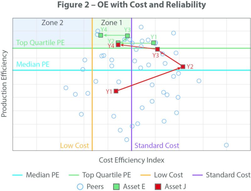
2. Journey to Operating Excellence
Assets outside of the operating excellence zone need to be targeted for improving performance on cost and/or reliability accordingly. For assets with a CEI lower than Standard Line and PE lower than the Top Quartile Line, increasing the spending budget with a focus on maintenance and/or labor should be the short-term goal. The purpose of this goal is to increase facility integrity and reliability, therefore improving on the PE. An example demonstrated in Fig. 2 shows how an asset (Asset J) improved its performance in the journey of four stages from Year 1 to Year 4 (Red Arrow Line). The asset starts with lower-than-average PE and lower-than-standard cost; the clear goal for improvement is on PE. Cost was increased significantly in Y2 to address reliability issues, and the elevated spending continued in Y3 to build on the sustainability. The final goal, as Y4 demonstrated, was to optimize the cost and maintain the top-level PE.
For assets with a CEI higher than the Standard Line and PE below the Top Quartile Line—especially those below the median line—the focus will still be improving the system integrity and reliability through best practices such as improving preventive maintenance and focusing on eliminating root causes of unplanned incidents. Cost optimization could be done in parallel only on the condition of not hurting system reliability.
For assets with a CEI higher than the Standard Line and PE above the Top Quartile Line, where reliability does not seem to be an issue, the focus will be on cost optimization. Logistics and field G&A will be the top categories to examine as empirical data generally show these categories have more room for savings. The focus on logistics should be on improving discipline by reducing the number of boat trips and the number of boats on contract, improving helicopter seat utilization, and optimizing trips. Optimization of maintenance and labor should focus on planning and execution, rather than simply cutting maintenance programs which could jeopardize system integrity. For example, spare capacity on mature assets with low utilization, including rotating equipment and especially compressors, can be scaled down, creating significant maintenance and operating cost savings.
Conclusion
Pursuing operating excellence is a long journey which requires an operator to also use proper KPIs and quality data. Proper benchmarking is proven to be an excellent tool to help companies embark on this journey to identify performance gaps and to align their operations with the best practices of the top operating performers.
Still, we see the need for the creation of an overall sustainability metric for performance comparison purposes that can provide an empirical linkage to reliability. The linkage between reliability and HSE/process safety management performance is intuitive; the most dangerous times in a facility are startups and shutdowns, and production losses often are associated with component failures that also create hazards and risks.
Those strategies and actions which deliver high reliability in a cost-efficient, sustainable, and safe manner fall under our definition of operations excellence. It is our goal to link not only these metrics but be able to empirically compare performance. This will allow us to provide guidance to the client group on which common actions are necessary to deliver the greatest business value. To date, our empirical observations reinforce our belief that the pursuit of reliability and elimination of system defects is the most prudent course of action.